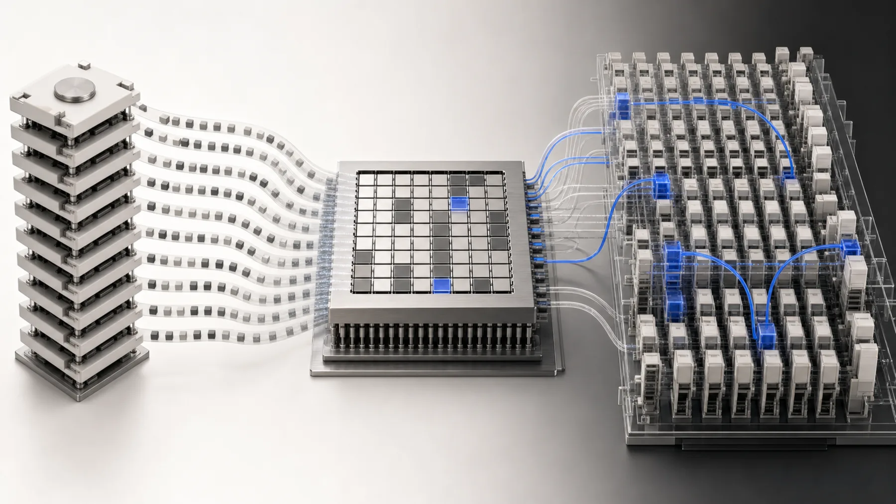
technology
22580: From GPT-2 to Kimi3, Explained
How attention and memory research transformed a 124M GPT-2 baseline into Kimi K3's hybrid 2.8T architecture.
Read MoreHow sparse attention, persistent CUDA kernels, four-step distillation, and NVFP4 turn a 133-second pipeline into near-real-time video generation.
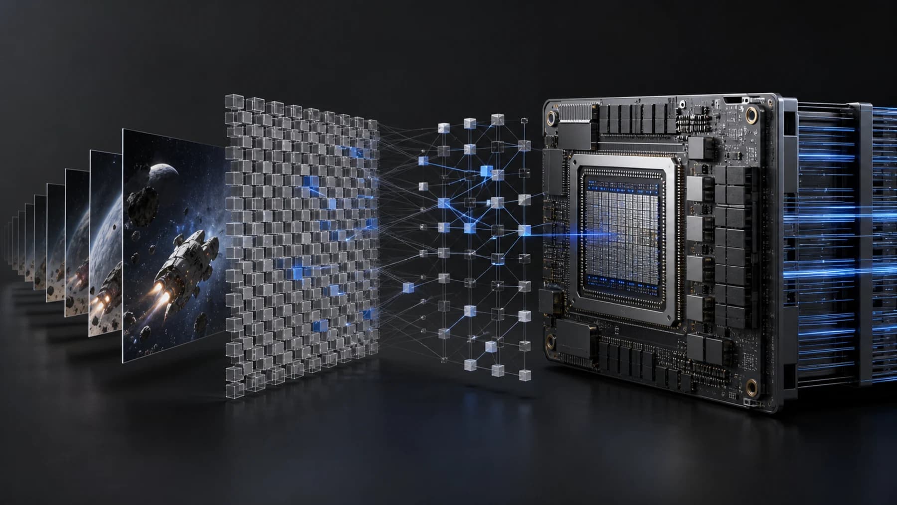
Baseten's public engineering report documents how its team moved Wan2.2 from a slow research runtime toward an interactive video system. The report and its released benchmark artifacts connect profiling, trainable sparse attention, kernel engineering, post-training, and low-precision inference.
This literature review reconstructs that work in a more explicit systems narrative. It cross-checks the headline against the Wan and VSA research, FlashAttention-4, NVIDIA's NVFP4 documentation, and Baseten's released production-shaped benchmark tensors.
Evidence status: Baseten's public product report gives 2.75 seconds per 480p clip and a 53.6x improvement. These are vendor-reported measurements on a B200, not an independently reproduced industry benchmark. The mechanisms are broadly documented, but the final checkpoint and complete custom runtime were not published with a one-command reproduction recipe.
Baseten's report begins near 133 seconds for one 832 x 480 video with 81 frames and ends at 2.75 seconds per clip on one NVIDIA B200, a reported 53.6x improvement over its baseline. It attributes the gain to three multiplicative groups:
| Optimization group | Baseten's reported contribution | Main trade-off |
|---|---|---|
| Four-step timestep distillation | About 20x | Lossy, with more risk on motion, physics, and consistency |
| Custom kernels and fusion | About 1.5x | Shape-specific engineering and hardware dependence |
| NVFP4 linear layers | About 1.5x | Quantization error and Blackwell dependence |
The official page states a cost reduction from five cents to less than one-sixth of a cent per video, not a general cloud price per second of output.
This distinction matters. A warm kernel path excludes model provisioning and weight download. A product user also experiences queueing, input moderation, text encoding, VAE decode, output checks, storage, and network delivery. Our AI inference latency guide explains why a kernel number, a warm model number, and user-visible latency need separate names.
Wan2.2 belongs to the diffusion-transformer family. The open Wan2.2 repository and the Wan technical paper describe a model family that denoises compressed video latents rather than generating pixels one after another. The T2V-A14B system uses a Mixture-of-Experts design so different experts specialize across the denoising trajectory.
For the report's 480p workload, the spatial latent is patchified into a grid of 30 x 52 tokens. Eighty-one output frames become 21 positions along compressed time. Before padding, the self-attention sequence therefore contains:
30 x 52 x 21 = 32,760 tokens
Dense self-attention compares every query token with every key token. One head would conceptually produce more than one billion scores because 32,760² is about 1.07 billion. The recorded workload uses 40 heads with head dimension 128. Even though FlashAttention avoids storing the full score matrix, it cannot avoid doing all dense query-key and probability-value work.
The reported profile placed self-attention above 60 percent of runtime. One dense attention call took about 17 ms. With 40 transformer blocks, many denoising steps, and classifier-free guidance, that small-looking latency is paid thousands of times. The optimization target was therefore not the model in the abstract. It was a repeated, measured hot path.
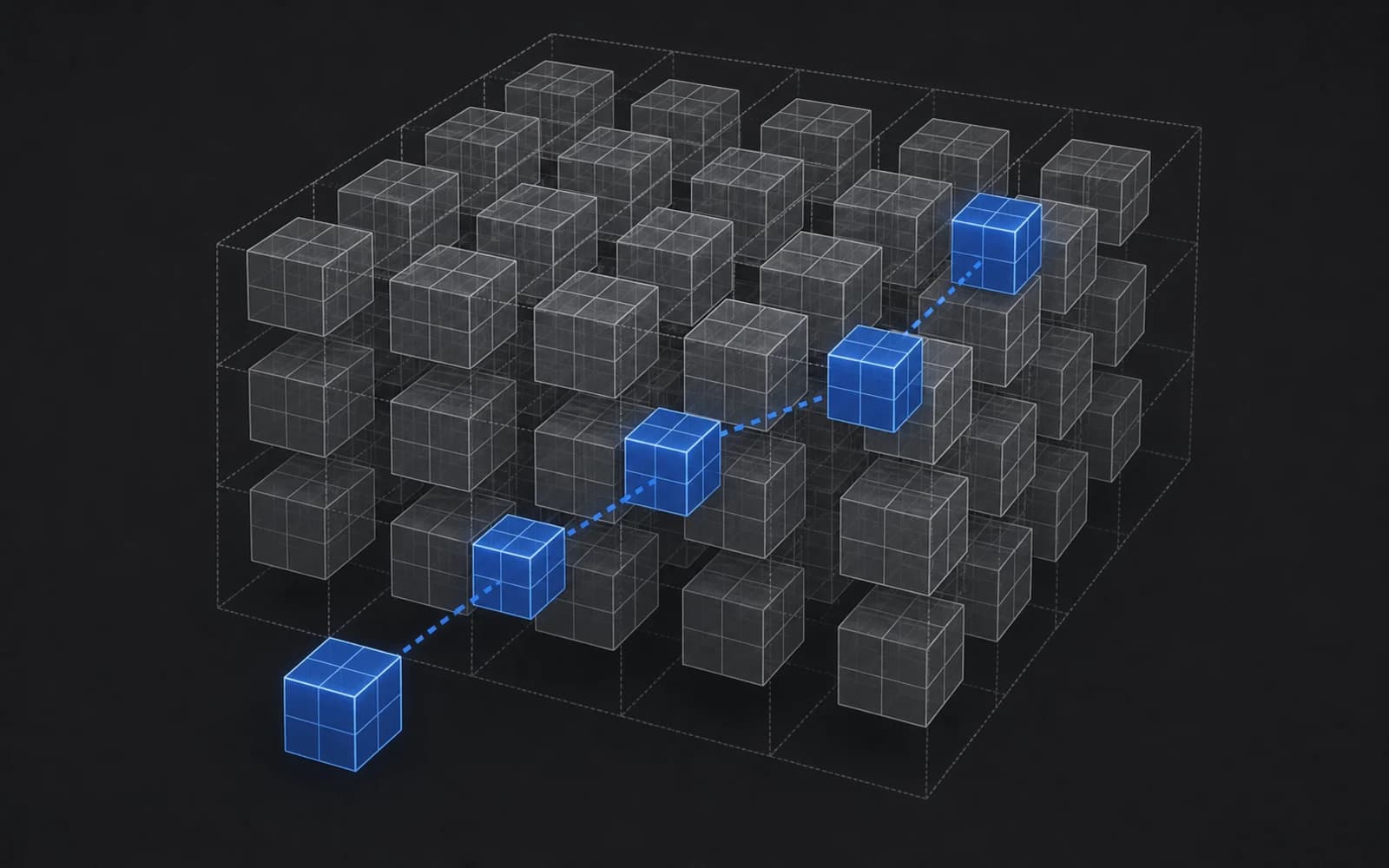
The central algorithm comes from Hao AI Lab's Video Sparse Attention research and FastVideo implementation. VSA exploits the observation that attention maps in video diffusion are often structured and sparse. A token usually needs a limited set of spatially or temporally related regions, not equal access to the entire clip.
The implementation groups the 3D token grid into 4 x 4 x 4 cuboids, each holding 64 tokens. Padding expands the conceptual 21 x 30 x 52 volume to 24 x 32 x 52, which explains the production QKV sequence length of 39,936. The number of cuboids is:
ceil(21/4) x ceil(30/4) x ceil(52/4) = 6 x 8 x 13 = 624
VSA then uses two connected branches:
At 87.5 percent sparsity, the kernel skips seven-eighths of the candidate cuboids and selects 78 of 624. Sparsity here means the fraction skipped. It does not mean 87.5 percent of output values become zero, and it does not reduce every part of the model by the same factor.
The block size is a quality and efficiency contract. Larger blocks reduce ranking detail. Smaller blocks increase selection overhead and reduce the work saved by each skipped block. The implementation uses 4 x 4 x 4 as the trained operating point and reports degradation with coarser grouping.
This is not a training-free mask attached after export. The coarse branch introduces gates that the original Wan2.2 checkpoint did not learn. The published method initializes those gates at zero and trains a sparse student against a frozen dense teacher. It combines latent-space mean-squared error with a CLIP embedding loss after VAE decoding, then also unfreezes student attention weights.
Hao AI Lab calls the broader method sparse distillation. Its FastWan description explains why trainable sparsity is useful when diffusion is compressed to very few steps. Heuristic masks often rely on redundancy across many denoising steps. With only one to four steps, that redundancy mostly disappears. The sparse student must learn which blocks remain important under the distilled trajectory.
This makes the checkpoint part of the runtime. You cannot copy only the CUDA kernel, point it at an arbitrary dense Wan model, and expect the same quality or selected-block distribution.
Before optimizing CUDA, the engineering analysis estimates a lower bound. Each query cuboid selects 78 key and value cuboids. Pairing two 64-token cuboids lets the kernel issue a 64 x 128 x 16 matrix-multiply-accumulate instead of a less efficient 64 x 64 form. Across 624 query cuboids and 40 heads, one launch covers 24,960 output tiles.
The rough compute demand is about 3.35 TFLOPs per attention launch after discounting padded tokens. The corresponding streamed K and V traffic is estimated near 64 GB. Under the assumed B200 tensor throughput and 19 TB/s L2 bandwidth, compute suggests about 2.86 ms while data delivery suggests about 3.35 ms. Perfect overlap cannot beat the slower bound.
This estimate is valuable even if simplified. It says a 7.5 ms Triton kernel still has headroom, but a 1 ms target would be physically inconsistent with the stated workload and bandwidth assumptions. A roofline is a feasibility check, not a promise.
The most instructive part of the engineering record is that several sophisticated changes made performance worse before the final pipeline emerged.
| Revision | Main change | Reported latency |
|---|---|---|
| Triton reference | Production block-sparse baseline | 7,444-7,503 µs |
| CUDA 1 | Direct SM100 port using MMA, TMA, and tensor memory | 9,169 µs |
| CUDA 2 | Producer-consumer pipeline and deeper staging | 11,553 µs |
| CUDA 3 | Fixed reference max to remove repeated rescaling | 10,788 µs |
| CUDA 4 | Separate probability-value warp group | 8,641 µs |
| CUDA 5 | More softmax worker groups | 7,779 µs |
| CUDA 6 | Independent K and V production | 6,564 µs |
| CUDA 7 | Move the top-K index list into shared memory | 6,374 µs |
| CUDA 8 | Fuse scale and sum with FMA | 5,841 µs |
| CUDA 9 | Prefetch upcoming shared-memory indices | 5,294 µs |
| CUDA 10 | Persistent CTAs to reduce fill and drain | 4,719 µs |
The first CUDA port was slower because using the right instructions is not the same as keeping the hardware busy. The initial algorithm serialized tile fetch, matrix multiplication, softmax, rescaling, and output accumulation. The producer-consumer rewrite added concurrency but consumed enough shared and tensor memory to reduce occupancy to one CTA per streaming multiprocessor. Lost occupancy exposed pipeline bubbles that two resident CTAs had previously hidden.
The FlashAttention-4 paper describes the same architectural pressure. On Blackwell, tensor-core throughput grew faster than shared-memory bandwidth and exponential-function throughput. Once matrix multiplication becomes extremely fast, softmax, memory movement, synchronization, and pipeline scheduling become first-order bottlenecks.
The custom VSA kernel assigns distinct warp groups to overlapping jobs: TMA producers stage Q, K, and V tiles in shared memory; asynchronous tensor operations produce score tiles in tensor memory; softmax workers consume those score tiles; another group launches the probability-value multiplication. Triple buffering lets later K and V tiles arrive while earlier tiles are being transformed and accumulated.
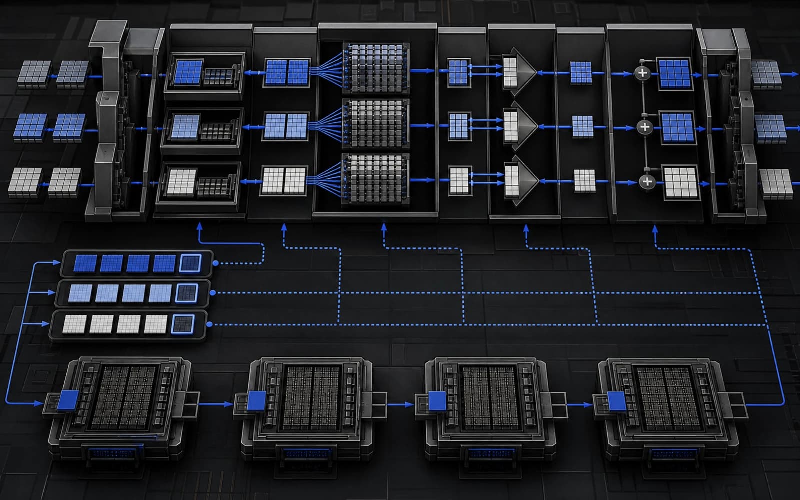
Separating K production from V production was especially important because they are consumed at different moments. A shared barrier kept memory occupied after K was finished simply because V was still live. Independent lifetimes let the pipeline recycle staging space sooner.
Online softmax normally maintains a running row maximum. When a later tile contains a larger maximum, the accumulated denominator and output must be rescaled. That is mathematically exact and numerically stable, but the repeated tensor-memory read, rescale, and write are expensive.
The optimized path instead fixes the subtraction constant from the first selected tile. Softmax probabilities are unchanged by subtracting any common constant, so the algebra remains exact. The risk is numerical: if a later score is much larger, an exponential can overflow in the chosen precision. The authors report that their diffusion workloads stayed inside a safe range.
This assumption must be tested on captured production tensors, not friendly random inputs. Baseten later published a Wan2.2 VSA benchmark dataset with real 832 x 480, 81-frame tensors and an explicit overflow outlier. Its card reports that a naive one-pass softmax without row-max subtraction produces 833,360 non-finite values in one of 40 heads on that capture. That does not automatically invalidate the optimized scheme, but it shows why a deployable implementation needs adversarial numerical cases, a tolerance contract, and a safe fallback.
The original launch assigns one CTA to one query tile. Each CTA fills its staging ring, reaches steady state, drains the ring, and exits. With 24,960 tiles on a B200, the GPU processes many waves of CTAs. Every wave repeats the same under-filled beginning and tail.
The persistent version launches roughly one CTA per streaming multiprocessor and keeps each CTA alive in a work loop. As one query tile finishes, the CTA pulls the next tile without tearing down the entire pipeline. The engineering analysis estimates about 15 percent combined fill and drain loss before this change. Measured tensor-core utilization rises from 62 to 71 percent, and latency falls from 5.294 to 4.719 ms.
Persistent kernels are not free. They can complicate scheduling, fairness, cancellation, and coexistence with other GPU work. They are strongest when shapes are stable, work is abundant, and the kernel owns the device long enough to amortize its residency.
After attention becomes faster, smaller operations become visible in the profile. Eager PyTorch can express RMSNorm, Adaptive LayerNorm modulation, and a gated residual add as several kernels. Each intermediate is written to and read from high-bandwidth memory, and each operation pays a launch cost.
The runtime fuses these sequences into Triton kernels so each tensor is loaded once, transformed through several elementwise or reduction stages, and stored once. The report cites 640 Q/K normalization instances across one four-step run. Fusion therefore saves both memory traffic and hundreds of launches.
The lesson is Amdahl's law in practice. A fused norm looks minor when dense attention dominates. Once sparse attention removes that bottleneck, the same norm can limit end-to-end progress. Optimization must return to the full trace after every major win.
Kernel work alone cannot turn more than two minutes into less than three seconds. The largest gain comes from reducing the denoising trajectory from roughly 40 to 80 steps to four. Baseten reports this moves generation from above 120 seconds to about six seconds before the later runtime optimizations.
The training recipe uses DMD2, which trains a student generator to match the teacher's output distribution rather than copying every individual denoising transition. A trainable fake score model helps estimate the student's current distribution, and an adversarial discriminator pushes local detail. For long video sequences, the training stack uses sequence parallelism so attention state is distributed across devices.
This speedup is explicitly lossy. Baseten notes more risk of artifacts, weak physical behavior, and temporal inconsistency in active scenes. A serious evaluation needs prompt strata, motion categories, temporal metrics, human pairwise review, and failure-rate reporting. Attractive cherry-picked clips are not a quality benchmark.
For the product consequences of generation speed, provenance, review, and delivery, see our AI video production workflow guide.
Once attention is sparse and denoising has only four steps, linear layers account for more of the remaining DiT compute. The runtime moves attention projections, feed-forward projections, and the VSA coarse gate to NVFP4. The actual QK and probability-value attention matrix multiplications remain in BF16.
NVIDIA's NVFP4 technical description defines a 4-bit E2M1 value, an E4M3 FP8 scale shared by each 16-value micro-block, and a global FP32 scale for the tensor. This two-level scaling gives more local range adaptation than a single scale and reduces weight memory substantially.
Selective precision is the important idea. The system does not force every operation into four bits. Large linear GEMMs gain from Blackwell's FP4 tensor throughput and reduced data movement. Numerically sensitive attention reductions stay in BF16. Quality still needs to be measured on the video checkpoint because language-model NVFP4 results cannot prove video fidelity.
The final runtime is a stack, not one world-record kernel:
| Layer | What changes | What it buys |
|---|---|---|
| Model trajectory | 40-80 denoising steps become 4 | The dominant order-of-magnitude reduction |
| Attention algorithm | Dense attention becomes learned block-sparse attention | Less QK and probability-value work |
| Attention kernel | Blackwell-specific asynchronous pipeline | Better overlap and resource utilization |
| Launch structure | Persistent CTAs | Less repeated fill and drain |
| Elementwise graph | Norm and residual fusion | Fewer launches and HBM round trips |
| Numeric format | Selected linear layers use NVFP4 | Higher GEMM throughput and lower data movement |
Multiplicative gains only compose when each measurement uses the same workload and quality target. If distillation changes the sequence distribution, kernel shapes or sparsity can change. If quantization changes top-K selection, the sparse kernel sees different work. End-to-end benchmarking is therefore the arbiter, not multiplication of isolated microbenchmarks.
An engineering team evaluating a similar claim should freeze the following contract before tuning:
Workload: exact checkpoint, prompt set, resolution, frame count, FPS, sampler, guidance, denoising steps, VAE, text encoder, sparsity, block shape, batch size, and random seeds.
Runtime: GPU SKU, clocks, power cap, driver, CUDA, PyTorch, compiler versions, warmup count, graph capture, synchronization points, and whether text encoding and VAE decode are included.
Kernel correctness: compare output and log-sum-exp tensors against a trusted reference, include padded edge blocks, duplicated top-K indices, all-full blocks, extreme values, overflow captures, and multiple denoising steps.
Quality: stratify prompts by camera motion, object motion, contact physics, text, faces, scene cuts, and long-range identity. Report temporal consistency and human preference with confidence intervals, plus the rate of severe failures.
Operations: report p50 and p95 warm latency, cold start, queue delay, throughput at offered load, cancellation behavior, GPU utilization, energy, and cost per completed acceptable clip.
The released Baseten tensor captures are a strong starting point for the kernel layer because they prevent synthetic inputs from hiding irregular top-K patterns. They are not a substitute for checkpoint-level and video-level evaluation.
First, profile before selecting an optimization. The winning project began with self-attention consuming most of the trace, not with a preference for CUDA.
Second, hardware balance matters more than peak FLOPs. On Blackwell, extremely fast tensor cores make exponentials, shared memory, synchronization, and occupancy visible. The right kernel is a schedule for all of those resources.
Third, regressions are evidence. The slower producer-consumer revisions revealed occupancy and resource-lifetime problems that a polished final diagram would hide.
Fourth, algorithm, checkpoint, kernel, and numeric format form one system. Learned sparse gates determine kernel inputs. Distillation changes the trajectory. Quantization changes values. Optimizing one layer while treating the others as fixed can produce a fast but invalid result.
Finally, near-real-time generation is a product threshold, not merely a benchmark. A 2.75-second clip can support a human loop of prompt, inspect, adjust, and retry. Production still needs scalable capacity, cold-start control, moderation, observability, and provenance. Fast inference creates a usable loop only when the surrounding system can sustain it.
This article was reviewed on July 31, 2026. Primary and first-party sources:
The two technical illustrations and cover on this page were created for ZharfAI as explanatory editorial artwork. They are conceptual, not profiler screenshots or die-accurate hardware diagrams.
How attention and memory research transformed a 124M GPT-2 baseline into Kimi K3's hybrid 2.8T architecture.
Read More
How affective computing interprets voice, face, and behavior—and why consent, bias, clinical validation, and human oversight determine whether emotion AI is safe.
Read More
How event-driven chips and brain-inspired architectures could reduce AI energy use—and where benchmarks, software maturity, and manufacturing still limit adoption.
Read MoreGet in touch with our team to discuss how we can help your business.