22580: From GPT-2 to Kimi3, Explained

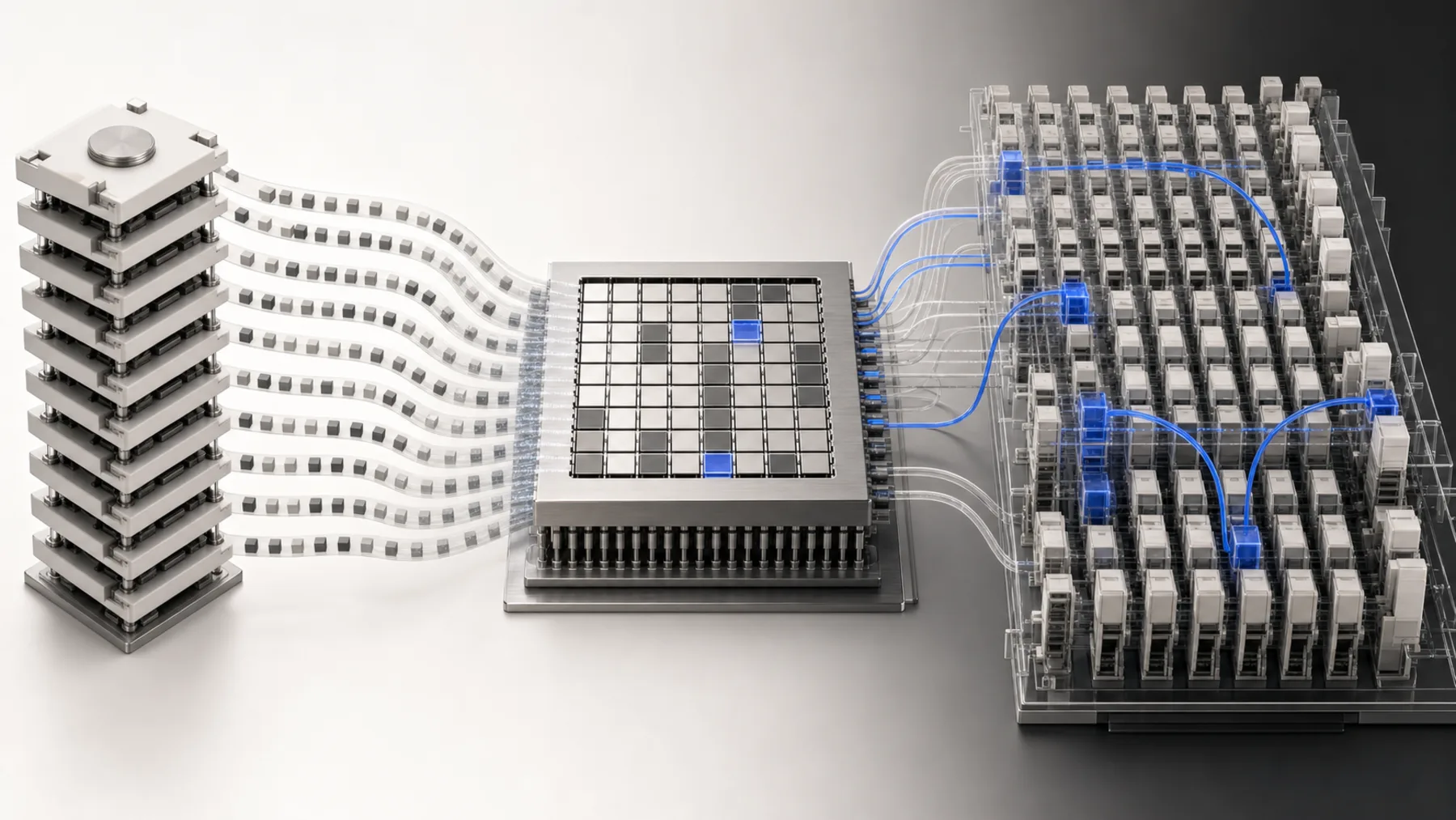
Ali Taha's worklog, 22580: From GPT2 to Kimi3, Explained, is a code-first tour through seven years of language-model architecture. It starts with a small GPT-2 implementation, follows the pressure created by long sequences and growing KV caches, and ends inside Kimi K3's hybrid system of recurrent memory, periodic softmax retrieval, sparse experts, and depth-wise attention.

This technical literature edition reconstructs the complete argument in a more explicit sequence. It cross-checks the worklog against Moonshot AI's official Kimi K3 release, the original GPT-2 report, and the papers behind linear attention, DeltaNet, Gated DeltaNet, Kimi Delta Attention, and Attention Residuals.

Evidence status: architecture dimensions and model counts below come from Moonshot AI's official report. The explanatory path and several implementation observations come from Taha's worklog. Performance figures such as 6x decode throughput or 2.5x scaling efficiency are author-reported results from the cited model papers, not universal guarantees for every sequence length, batch size, kernel, or device.

What the number 22,580 means

The title is mathematically real, but only under a specific comparison:

2.8 trillion / 124 million = 22,580.6

The denominator is the compact GPT-2 configuration used by the worklog and by Karpathy's nanoGPT implementation: 12 layers, 12 attention heads, and a 768-dimensional hidden state. nanoGPT counts that configuration at about 124 million parameters. OpenAI's original GPT-2 report listed the small model at 117 million and the largest GPT-2 at roughly 1.5 billion, so "22,580 GPT-2s" is not a ratio to GPT-2 XL.

There is a second distinction. Kimi K3 has 2.8T total parameters, but its sparse Mixture-of-Experts path activates 104B parameters per token. The active-parameter ratio to the 124M baseline is therefore about 839x, not 22,580x.

The number is a useful scale marker, not a measure of intelligence, training compute, energy use, latency, or quality. The deeper story is how the model uses memory and capacity.

GPT-2 established the decoder-only baseline

GPT-2 is a stack of decoder blocks. Token and position embeddings enter the stack. Each block applies causal self-attention and an MLP, with residual connections carrying information through depth. A final normalization and language-model head produce vocabulary logits.

x = token_embedding(tokens) + position_embedding(positions)
for block in transformer_blocks:
    x = x + block.attention(block.norm_1(x))
    x = x + block.mlp(block.norm_2(x))
logits = language_model_head(final_norm(x))

The 124M configuration is small enough to understand as a complete program:

Autoregressive generation consumes only the logits at the newest position. Without caching, the model would recompute projections for every earlier token after each new token is appended. A KV cache avoids that duplication by retaining the keys and values produced at previous positions.

That optimization creates the next bottleneck: the cache grows with sequence length. Each new query still needs to compare itself with an expanding history, and the keys and values must be read from memory.

Softmax attention remembers tokens explicitly

For one attention head, standard causal attention can be summarized as:

Attention(Q, K, V) = softmax(QKᵀ / √d) V

During training or prompt prefill, a sequence of length N forms an N x N score structure, so arithmetic grows quadratically with sequence length. FlashAttention improves the memory traffic and avoids materializing the entire score matrix, but it does not remove all query-key comparisons.

During cached decoding, only one new query is produced at each step. The arithmetic for that step grows linearly with the number of cached tokens, while the KV cache itself also grows linearly. This distinction matters:

Softmax attention is expressive because it can retrieve an individual earlier token with high precision. Its weakness is that the model pays for an explicit token history.

Linear attention collapses history into a fixed state

The Linear Transformers paper changes the order of operations. Softmax applies a nonlinearity after query-key interaction, which prevents simple reassociation. Linear attention applies a nonnegative feature map to queries and keys separately:

φ(Q) (φ(K)ᵀ V)

The model can update a fixed-size state instead of appending every key and value:

state = state + outer(phi(key), value)
normalizer = normalizer + phi(key)
output = phi(query) @ state
output = output / (phi(query) @ normalizer)

For head dimension d, the associative state is roughly d x d, independent of sequence length. Decode no longer scans an unbounded KV list. New information is folded into the same matrix, producing constant-state recurrent inference.

The price is compression. The state is not a bag of perfectly isolated token slots. Multiple key-value associations share a finite matrix, and a simpler kernel feature map is less expressive than exact softmax retrieval.

A finite associative memory eventually interferes

Additive linear attention writes every new association into the same state:

S_t = S_(t-1) + k_tᵀ v_t

When keys are well separated, a later query can recover a useful approximation of the matching value. As more associations accumulate, similar key directions overlap. Old and new facts interfere because nothing is removed.

The Fast Weight Programmers paper frames this as an over-capacity problem. A finite memory needs a way to decide what to retain, what to replace, and what to forget. Pure addition has no eviction policy.

This is the first major architectural shift in the worklog:

The delta rule turns writing into editing

DeltaNet reads the value currently stored at a key before writing. It then writes only the difference between the desired value and the retrieved old value:

old_value = key @ state
correction = beta * (new_value - old_value)
state = state + outer(key, correction)
output = query @ state

In compact form:

S_t = S_(t-1) + β_t k_tᵀ (v_t - k_t S_(t-1))

β_t is a learned write strength. Near zero, the token barely changes memory. Near one, the update strongly replaces the association along the current key direction.

This is more than a cache optimization. It changes the state from an append-only accumulator into an editable associative memory. If a key retrieves a stale value, the model can subtract that value and write a corrected one without clearing every unrelated association.

Chunkwise DeltaNet makes the recurrence trainable on GPUs

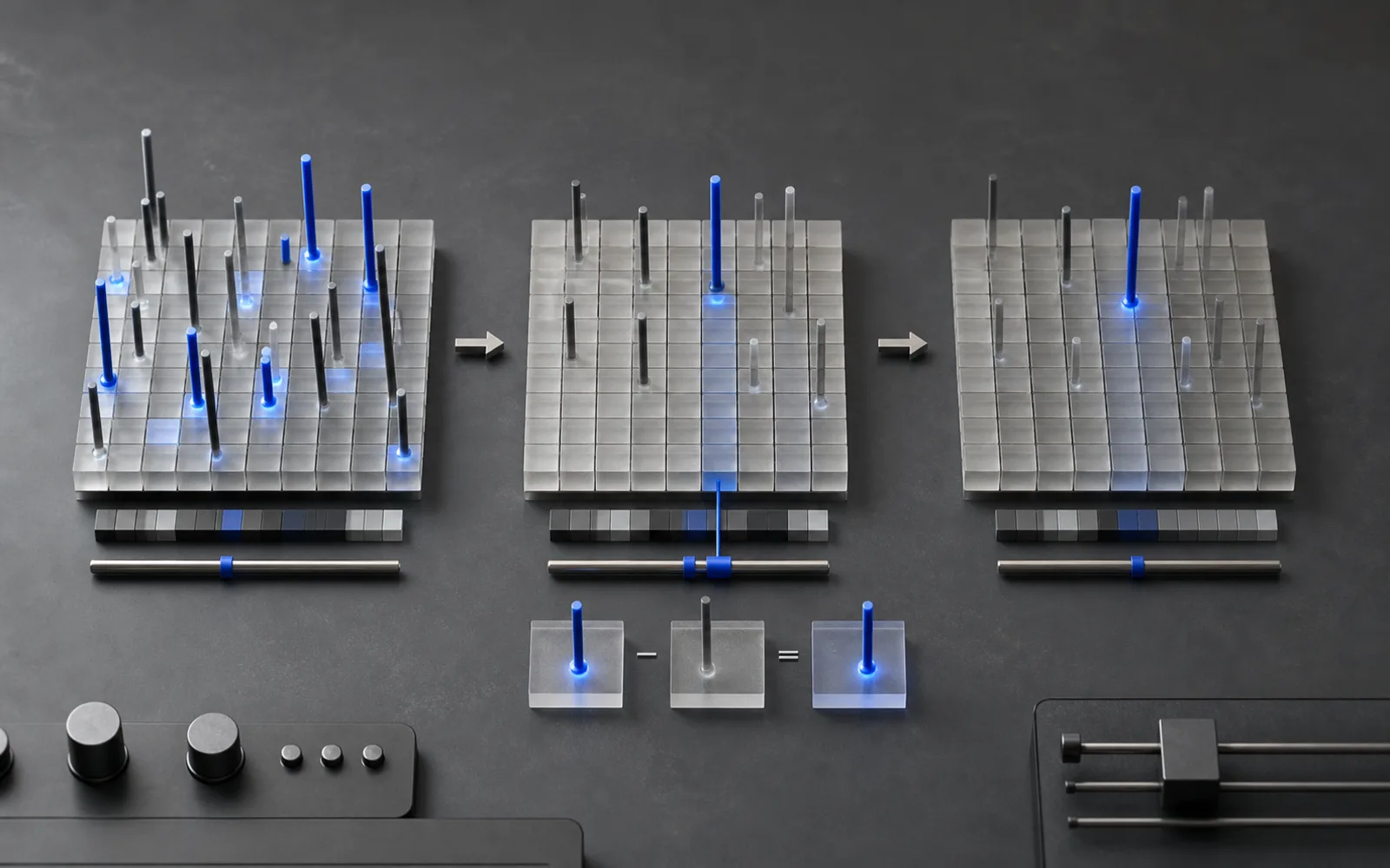
The direct delta recurrence is sequential. Token t must read S_(t-1) before it can compute its correction, which appears incompatible with the wide matrix operations GPUs prefer.

The parallel DeltaNet algorithm rewrites the recurrence with products of generalized Householder transition matrices and a compact WY representation. The sequence is split into chunks of C tokens:

• Inside a chunk, masked matrix operations handle token interactions in parallel.
• Between chunks, a recurrent state carries the compressed history.
• Auxiliary matrices encode the corrections that would otherwise require a token-by-token loop.

The work can be understood as two terms:

approximately 2Ld² + 2LCd

L is sequence length, d is head dimension, and C is chunk length. Full attention appears when C approaches L. A very small C reduces arithmetic but may underuse tensor cores. Practical chunk sizes such as 64 or 128 balance recurrent efficiency with hardware-friendly matrix tiles.

This is a recurring systems lesson: fewer FLOPs do not automatically mean lower wall-clock time. The algorithm must expose enough regular matrix work to keep the GPU busy.

Gated DeltaNet adds controlled forgetting

The delta rule can replace one association when a matching key arrives, but it has no general mechanism for clearing a stale context. Gated DeltaNet combines targeted delta updates with a data-dependent decay:

S_t = α_t (I - β_t k_tᵀk_t) S_(t-1) + β_t k_tᵀv_t

α_t controls how much previous memory survives:

• α_t near one preserves history and behaves like the delta rule.
• α_t near zero rapidly clears old state.
• Intermediate values create gradual forgetting.

The gate and the delta correction solve complementary problems. The gate erases broadly when context changes. The delta term edits a particular key-value association.

Because decay compounds across time, an association written at position x reaches a later position multiplied by the intervening gates. Efficient chunkwise implementations therefore need cumulative products as well as the DeltaNet correction machinery.

Kimi Delta Attention makes forgetting finer

The Kimi Linear paper extends Gated DeltaNet with Kimi Delta Attention, or KDA. Instead of one scalar decay for an entire head, KDA learns finer per-channel decay. Different features can retain or forget information at different rates.

Kimi Linear does not replace every softmax layer. It uses a hybrid:

• KDA layers provide constant-state recurrent memory.
• Multi-Head Latent Attention layers periodically recover precise token-level context.
• Sparse Mixture-of-Experts layers increase capacity without activating every parameter.

In the paper's controlled experiments, the 48B-total / 3B-active Kimi Linear model outperformed a full-MLA baseline using the same training recipe. The authors report up to 75 percent lower KV-cache use and up to 6x decode throughput at a one-million-token context. Those are architecture-and-system results under the paper's setup, not a claim that every KDA layer is always six times faster.

The hybrid is important because finite-state memory and full retrieval fail differently. KDA is efficient but must compress. MLA is more expensive but can inspect the token context directly.

Kimi K3 scales the hybrid into a 2.8T MoE

Moonshot AI's official model summary describes Kimi K3 as a 93-layer, open-weight, native multimodal model with a one-million-token context window.

The 69-to-24 attention split forms a repeating rhythm: three KDA layers for every gated-MLA layer across 23 four-layer macrocycles. The first feed-forward layer is dense; later layers use the sparse latent MoE path.

This arrangement spends explicit retrieval where compression alone would be risky, while recurrent layers handle most sequence mixing with constant state.

Latent MoE separates capacity from per-token work

Kimi K3 routes each token to 16 of 896 routed experts and also uses two shared experts. The full parameter set contributes to model capacity, but only a small fraction of expert weights participates in one token's forward pass.

The expert computation operates in a compressed latent width rather than the full model width. That design reduces expert-side arithmetic and communication, helping Kimi K3 activate 104B parameters from a 2.8T model.

Sparse routing creates its own systems problems:

• Tokens must be balanced across expert devices.
• Expert weights and activations need efficient communication.
• Popular experts can become hotspots.
• Capacity can be large even while active compute remains bounded.

This is why total parameters, active parameters, FLOPs, memory footprint, and latency should be reported separately.

SiTU and gated MLA refine the data path

Kimi K3 uses the SiTU-GLU activation. In simplified form, the gate applies both a bounded tanh term and a sigmoid, controlled by learned scale parameters:

gate, up = split(x)
activated_gate = beta * tanh(gate / beta) * sigmoid(gate)
output = activated_gate * up

The worklog notes a practical tension: a mathematically attractive activation can be slower than an older path until its operations are fused into an efficient kernel. Architecture and implementation cannot be evaluated independently at this scale.

The periodic MLA layers are also gated. A learned signal controls how much retrieved attention output enters the residual stream. This lets the model suppress unhelpful retrieval instead of injecting every attended feature at full strength.

AttnRes lets layers retrieve across depth

Standard PreNorm transformers accumulate residual outputs with fixed weight:

h_l = h_1 + Σ f_i(h_i)

As depth grows, hidden-state magnitude can increase and the contribution of an individual layer can become diluted. Different sublayers also receive the same accumulated mixture even when they need different earlier representations.

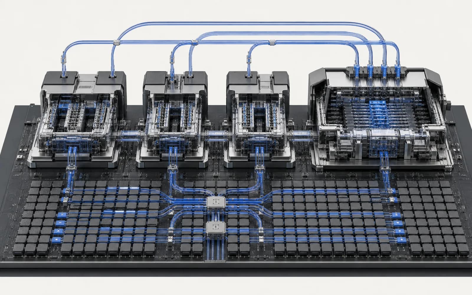
The Attention Residuals paper replaces the fixed sum with softmax attention over earlier residual states. Each layer learns a query. Earlier states provide keys and values. The current layer then forms a content-dependent weighted combination of the depth history.

Full AttnRes would make every layer attend to every earlier layer, which adds memory and communication overhead. Block AttnRes groups several layers into one stored representation. Kimi K3 uses a block size of 12, so depth retrieval happens at a manageable granularity.

KDA and AttnRes address two different axes:

This is the strongest idea in the worklog. Modern architecture is not one attention trick. It is a set of selective memory systems operating across time, token context, depth, and expert capacity.

The architecture changed what memory means

The evolution can be read as a sequence of specific failures and repairs:

The trajectory is not "transformers became 22,580 times larger." It is "memory became editable, forgetful, hybrid, sparse, and depth-selective."

What the headline does not prove

Several caveats keep the comparison honest:

1. Parameter count is not compute. Kimi K3 activates 104B parameters per token, not all 2.8T.
2. GPT-2 has several sizes. The 22,580 ratio uses the 124M small configuration, not GPT-2 XL.
3. Long context is not perfect recall. A one-million-token window defines capacity, not guaranteed retrieval accuracy at every position.
4. Linear-time does not mean free. Fixed-state methods still perform matrix work and require specialized kernels.
5. Hybrid models keep softmax attention. Kimi K3 reduces dependence on full retrieval; it does not eliminate it.
6. Vendor benchmarks need context. Throughput and scaling-efficiency claims depend on training recipe, precision, sequence shape, batching, and hardware.
7. Open weights do not make deployment simple. A 2.8T MoE still needs major storage, networking, expert parallelism, and inference engineering.

For practical serving, our AI inference latency guide explains why architecture, kernel speed, batching, and user-visible latency must be measured separately. Our small language models guide covers the opposite design point: reducing capacity so models can run near users. The Wan2.2 runtime study shows the same algorithm-system co-design pressure inside video generation.

A reproduction-oriented reading path

Readers who want to move from explanation to implementation can follow this order:

1. Implement GPT-2-small or inspect nanoGPT until Q, K, V, causal masking, residuals, and KV caching are concrete.
2. Implement normalized linear attention with a recurrent d x d state and compare its decode memory to a KV cache.
3. Add the delta correction and test repeated writes to the same key.
4. Read the chunkwise DeltaNet derivation and verify recurrent and chunkwise outputs against each other.
5. Add scalar decay, then inspect how Gated DeltaNet combines broad forgetting with targeted replacement.
6. Study KDA's per-channel transition and the hybrid KDA/MLA schedule.
7. Inspect Moonshot's Kimi K3 configuration and open model code before estimating deployment cost.
8. Treat kernel fusion, expert routing, quantization, and distributed communication as part of the architecture, not postscript optimization.

Useful tests include associative recall, repeated-key replacement, context switches, long-sequence numerical stability, recurrent-versus-chunkwise equivalence, expert load balance, and end-to-end decode memory.

Source notes and review date

This literature review was checked on July 31, 2026 against:

• Ali Taha's original X worklog
• Moonshot AI's official Kimi K3 repository and model summary
• OpenAI's GPT-2 technical report
• Karpathy's nanoGPT GPT-2 implementation
• Transformers are RNNs: Linear Attention
• Linear Transformers Are Secretly Fast Weight Programmers
• Parallelizing Linear Transformers with the Delta Rule
• Gated Delta Networks
• Kimi Linear
• Attention Residuals

The illustrations are original editorial diagrams created for this ZharfAI edition. They explain relationships and data flow; they are not official Moonshot AI architecture schematics.